
How to compute the Gamma index?
The function rt.gamma.index() or rt.chi.index() allows you to compute γ index or χ index to compare a 2D-3D measured dose map to a reference dose map. The following explanations concern how to use the functions when you want to compare 2D images.
- Loading data from RTimage
rt.gamma.index() and rt.chi.index() can directly use RTimage, first exported to espadon object of class volume : with the project.to.isocenter argument set to TRUE, the image will be projected onto the isocenter. However, make sure that the objects share the same frame of reference. If this is not the case, and you are sure that the images can be overlaid in the machine frame of reference, we advise you to put the images in the machine frame of reference.
library(espadon)

D.ref <- load.obj.from.dicom(ref.dcm)
D.meas <- load.obj.from.dicom(meas.dcm)

# check the differences in the frames of reference
D.ref$frame.of.reference == D.meas$frame.of.reference

# As needed, put in the frame of reference of the machine
D.ref <- vol.in.new.ref(D.ref, new.ref.pseudo = "reF.m",
                        T.MAT = ref.cutplane.add(D.ref ,ref.cutplane ="reF.m" ))

D.meas <-vol.in.new.ref(D.meas, new.ref.pseudo = "reF.m",
                        T.MAT = ref.cutplane.add(D.meas,ref.cutplane ="reF.m" ))


# check for differences in voxel sampling
# --> same number of voxels in the 3 directions
D.ref$n.ijk
D.meas$n.ijk
# --> same volume orientation
D.ref$orientation
D.meas$orientation

# If there are differences in voxel sampling, the grid of one volume must be
# resampled to the grid of the other volume.
D.meas <- vol.regrid(D.meas, back.vol = D.ref)

# coordinates of the point where the maximum dose is located :
coord <- as.numeric(get.xyz.from.index(which.max(D.ref$vol3D.data),D.ref))

par (mfrow = c (1, 2))
display.plane (top = D.ref, interpolate = FALSE, view.coord = coord[3])
display.plane (top = D.meas, interpolate = FALSE, view.coord = coord[3])
par (mfrow = c (1, 1)) - Loading data from csv file
If this export is a csv file, you also need to know the size of the detector pixels, projected onto the isocenter.
The following function creates an espadon “volume” class object, from csv file:
- csv.file argument represents the path of the image file,
- dxy is the interpixel distance, or the pixel size,
- you can define your description in the description argument : for example “reference” or “measured”.
- … : represents all added arguments to import a file from csv : header, sep …
vol.from.csv <- function (csv.file, dxy, modality, description = "", ...) {
  d <- as.matrix (read.csv (csv.file, ...))

  if (length(dxy) == 1) {
    pixel.dxyz <- c (dxy, dxy, 0)
  } else if (length(dxy) == 2){
    pixel.dxyz <- c (dxy, 0)
  } else {
      return (NULL)
  }
  map <- vol.create (n.ijk = c (ncol (d), nrow (d), 1),
                     dxyz = pixel.dxyz, ref.pseudo = "ref1",
                     alias = unlist (strsplit (basename (csv.file),"[.]"))[1],
		     modality = modality,
                     description = description)


  map$acq.date <- substr (file.mtime (csv.file), 1, 10)
  map$vol3D.data[,,1] <- as.array(t(d))
  map$max.pixel <- max (map$vol3D.data, na.rm = TRUE)
  map$min.pixel <- min (map$vol3D.data, na.rm = TRUE)

  return (map)
}
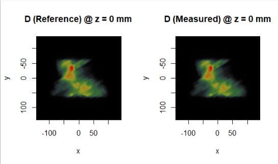
The measured and reference images can be converted into objects of the “volume” class and then displayed:
library (espadon)

file.ref <- file.choose()
file.meas <- file.choose()

D.ref <- vol.from.csv (file.ref, dxy = 0.22, modality = "D", description = "Reference")
D.meas <- vol.from.csv (file.meas, dxy = 0.22, modality = "D", description = "Measured")

par (mfrow = c (1, 2))
display.plane (top = D.ref, interpolate = FALSE, view.coord = D.ref$xyz0[1,3])
display.plane (top = D.meas, interpolate = FALSE, view.coord = D.meas$xyz0[1,3])
par (mfrow = c (1, 1))
- maximum reference value
The global gamma index is calculated with respect to a maximum reference value. To avoid outliers or image noise, it is possible to use the 99.99% quantile value, as well as the maximum value of the median filtered image. The following instruction performs this operation:
# maximum reference value with quantile
D.max <- as.numeric(quantile(as.numeric(D.ref$vol3D.data) , probs = 99.99/100, na.rm =TRUE))

# maximum reference value with median filtered image
D.max <- vol.median (D.ref)$max.pixel
- calculation and display of the gamma index
Then simply compute the γ index with the rt.gamma.index() function (here γ index 2%-3mm, with analysis threshold set at 5%), and display it with an appropriate palette. Note also that you can calculate the χ index with the rt.chi.index() function.
gamma <- rt.gamma.index(D.meas, D.ref, vol.max =D.max, analysis.th = 0.05,
                        dose.th = 0.02, delta.r = 3, local = FALSE)

gamma$gamma.info
     label value
1   <1 (%) 92.05
2      max  4.50
3     mean  0.51
4 >1.5 (%)  1.36
5 >1.2 (%)  4.04

# display
gamma.col <- c ("#00FF00", "#007F00", "#FF8000", "#FF0000", "#AF0000")
gamma.breaks = c (0, 0.8, 1, 1.2, 1.5, min (gamma$max.pixel, 10))

def.par <- par(no.readonly = TRUE)
layout (matrix (1:2, ncol = 2), width = c (3, 1), height = c (3, 3))
display.plane (gamma, view.coord = gamma$xyz0[1,3],
              bottom.col = gamma.col, bottom.breaks = gamma.breaks,
              bg = "blue", interpolate = TRUE)
display.palette (gamma.col, breaks = gamma.breaks, new.window = FALSE,
                 override.breaks = FALSE)

par (def.par)  # reset to default
