Histograms

Get started

Histograms computing is a basic function proposed by R. The espadon package adds the feature to compute these differential histograms over an imaging volume such as CT, MR, PT, rt-dose, and within a predefined area:

either by a region of interest (RoI) of an rt-struct file : histo.from.roi function
or by a selection by binary volume : histo.from.bin function.

To be able to simulate random shifts of the selection, or variations of contours, the histo.from.roi function includes Monte Carlo calculations, according to a normal distribution.

If the imaging volume is a dose distribution (from an rtdose file), it is then easy to calculate a cumulative histogram, called in this case dose-volume histograms or DVH, using the histo.DVH function.

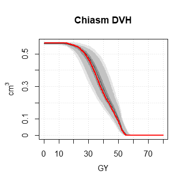
The functions display.dV_dx, display.DVH, display.DVH.pc allow to display pretty graphs, including the quantile zones 100%, 95% and 50% of the Monte-Carlo data.

In the following example, the patient folder contains a CT-scan files, a rt-dose file and a rt-struct file in which optic chiasm is outlined :

library (espadon)
patient.folder <- choose.dir ()
pat <- load.patient.from.dicom (patient.folder, data = FALSE)

S <- load.obj.data (pat$rtstruct[[1]])
CT <- load.obj.data (pat$ct[[1]])
D <- load.obj.data (pat$rtdose[[1]])

# resample D on the cut planes on which the chiasm has been outlined
D.on.CT <- vol.regrid (D, CT)

# Calculation of histogram with simulation of random displacements according to 
# a normal distribution of standard deviation 1 mm in all directions:
h <- histo.from.roi (D.on.CT, S, roi.name="chiasm", breaks = seq(0, 80, 0.1),
                     alias = "chiasm", MC = 100 )

DVH <- histo.DVH (h, alias = "Chiasm DVH")

display.DVH (DVH, MC.plot = TRUE, col = "#ff0000", lwd = 2)