3D Display

Get started

The espadon package has several 3D visualization features:

the display.3D.contour function displays the contours of the selected region of interest as described in the rt-struct.
the display.3D.stack function displays selected slices of the imaging volume.
the display.3D.sections function displays the frontal, sagittal and transverse view at a point.

These last 2 functions can use the same color palettes as the 2D visualization functions, except that a color can only be totally transparent or visible.

Thanks to the internal management of geometrical frames of reference, the different displays can be mixed, as shown in the example below:

library(espadon)
library(rgl)
pat.dir <- choose.dir () # patient folder containing mr, ct, rt-struct, and reg
pat <- load.patient.from.dicom (pat.dir)
S <- load.obj.data(pat$rtstruct[[1]])
CT <- load.obj.data(pat$ct[[1]])
MR <- load.obj.data(pat$mr[[1]])

bg3d ("black")
par3d (userMatrix = matrix (c(0, 0, -1, 0, -1, 0, 0, 0, 0, 1, 0, 0, 0, 0, 0, 1), ncol = 4), 
       windowRect = c(0, 50, 300, 300), zoom = 0.7)

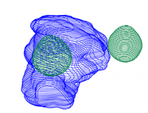
display.3D.contour (S, roi.sname = "eye", display.ref = CT$ref.pseudo, T.MAT = pat$T.MAT)
display.3D.stack (MR, k.idx = c(10,35,70, 105, 140,165), display.ref = CT$ref.pseudo, T.MAT = pat$T.MAT,
                  ktext = FALSE)
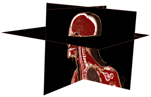
display.3D.sections (CT, cross.pt = c(0, 150, 0), col = pal.RVV (200, alpha = c(rep (0, 90), rep (1, 110))),
                     breaks = seq(-1000, 1000, length.out = 201), border.col = "#844A39")

play3d (spin3d (rpm = 4), duration = 15)